Accuracy of Results
The procedure described here can be handled for you, fully automatically by Simul8, but it is described here so that you can fully understand to principles involved.
Once some insights have been gained it is important to test the resulting ideas, especially if there are a number of competing ideas and it is difficult to see visually the best one. Remember that a simulation (usually) contains random numbers and if you are simulating a week's production when you explore the simulation visually, you may be seeing results that apply only to one week (perhaps a lucky week when few of the machines broke down!). A different week might give you slightly (or very) different results.
This procedure described here gives you a step-by-step way to ensure your results are valid. Even if you do not feel a need to go as far as calculating the statistics, you should do the first part and run the simulation with a number of different set of random numbers.
When using most simulation packages, if you set the time clock back to zero and re-run the simulation you will see exactly the same things happen on the screen, in the same sequence as the last time you ran it (despite the fact that the simulation contains random numbers to emulate 'real life'). This is because simulation packages use 'pseudo random numbers' that are generated mathematically and simply appear to be random. Each time the random numbers are re-started, the same sequence of numbers will be generated. This is very useful because it means you can re-watch a simulation several times to understand exactly what is happening, without the issue being clouded by the random numbers changing each time.
All simulation packages allow you to change the random numbers so you can also see what happens when the random numbers are different. They do this by allowing you to set the 'stream' of random numbers that will be used. Most packages have many thousands of 'streams' of random numbers built into them so there is no limit on the number of different weeks you can simulate in the factory.
But wait a moment - why are we only simulating a week's production? Why not a year, or an hour? What is the right length of time to simulate? The answer is simple. Simulate an amount of time that makes sense to your client in terms of the performance measure you are using. For example if you simulate the factory for a year and report to your client that you expect the factory to produce 14,500 boxes in a year this might be useful information in itself but might hide the information that any given week's production might be as low as zero or as high as 500. Conversely, your client may be unconcerned by information about the output in any given hour. Choose a time that makes sense to the client. The decision about what time to choose will become clearer when we see (next) what we will do with the information we get.
Lets assume we choose to simulate the factory for one week at a time and with each random number stream we get a different number of products completed by the end of the week. This information can be really useful to your client for making decision with - but it has to be presented in a useful and valid way for it to be of genuine use. This section is all about how to do this.
Once we get to this stage of a simulation study we are normally doing these runs and recording the results because we want to compare two or more alternative decisions that we cannot easily distinguish between visually. Lets assume we have two alternatives and we have run the simulation 30 times for each of these alternatives. For each run (of a week plus warm-up time) we have used different random numbers and obtained the following output figures:
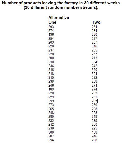
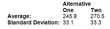
The results for alternative one are as low as 189 and as high as 315 with the figures for alternative two being 188 and 334. What one is best? The averages for the two alternatives are 245.8 and 270.5, so perhaps alternative two is best. There is so much overlap between the two, perhaps there is not really any difference between the two alternatives. Can your client really justify spending the extra £1million that alternative two will cost? What if the next 30 weeks (random number streams) average out the other way around? What will the genuine long term average really be?
A simple statistical procedure can help here. With limited time to do a limited number of simulation runs we cannot given our client a dead-accurate long term average, but if we could tell our client what range we expected the long term average to be inside this might be good enough.
In addition to the information we have so far we could calculate the standard deviation of the individual results:
But this only tells us the variability of the individual results. We are interested in how safe our average figure is. If we had time to do another batch of 30 runs, would its average be different? If we did 30 batches of 30 runs what would the variability of the averages be?
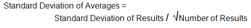
Fortunately for us there is a statistical relationship that applies here that provides a method of predicting the standard deviation of the averages from the standard deviation of the individual results - that we have just calculated.
In our case:

We can now calculate confidence limits for our average to report to our client.
As 95% of normally distributed numbers are within 2 standard deviations of their average then:
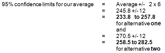
This means that we can say we are 95% confident that the true average for alternative one lies in the range 233.8 to 257.8 and also that we are 95% confident that the true average for alternative two lies in the range 258.5 to 282.5. So (again with 95% confidence) alternative two will produce more boxes in the long term (but not every week!)
A picture of this can be useful:
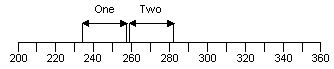
Showing this type of picture to your client can help understanding especially if you change the numeric production count information into profit or cost. The above picture shows that it is just possible to distinguish (statistically) between these two alternatives.
Of course the picture might show this:
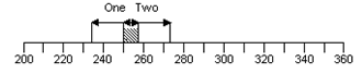
An overlap between the two ranges in that case:
- You cannot distinguish between the two alternatives. It is not reasonable to report any difference between them to your client because the average for alternative one could be as high as 257 and the average for alternative two could be as low as 254.
- You could do more runs because (take a look at the way the range is calculated) the larger the number of runs the smaller the predicted standard deviation of the averages: so the smaller the range. Of course this does not mean the two ranges will definitely separate if you do more and more runs - it simply means your figures are getting more and more accurate. You may move towards something like this:
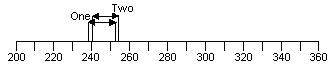
If this happened it would show there is no difference between the alternatives.
It is rarely necessary to do as many as thirty runs. If you do five runs and then do these calculations you will get an idea as to whether five is enough or whether you will need to do more. Even as few as five can be enough - see the note on statistical theory below.
To summarize the procedure:
- Do five runs of each of your alternatives, each run using a different random number stream.
- Calculate the average and standard deviation for each of your alternatives.
- Calculate the 95% confidence limit ranges for each alternative = Average +/- 2 x Standard Deviation /
 Number of Result
 - Draw these up on a picture like the one above to see what alternatives can be distinguished from each other, possibly changing the data to something more meaning full to your client (like £ or $).
- If ranges overlap do more runs to see if they separate.
A bit of statistical theory
This procedure only works if we know the averages are going to be 'normally' distributed. If we have at least 25 runs to calculate our average then this will be the case but fortunately for simulation users this is usually the case for smaller numbers of runs because the average will be normally distributed if the individual run results are normally distributed. These are (usually) normally distributed because they are, themselves, the combination of a large number (more than 25) individual events (the times between products leaving the factory). A statistical theory called 'central limit theorem' says that any number that is the total (or average) of a large number of other numbers will be normally distributed, whatever the distribution of the original numbers.